This reading deals with how to analyze the data from the experiment to determine the answer to the question you came up with experiment design.

 Let's talk about a simple, rough method for judging whether an experiment might support its hypothesis or not, if the statistics you're using are **means**.
The **standard error of the mean** is a statistic that measures how close the mean statistic you computed is likely to be to the true mean. The standard error is computed by taking the standard deviation of the measurements and dividing by the square root of n, the number of measurements. (This is derived from the Central Limit Theorem of probability theory: that the sum of N samples from a distribution with mean *u* and variance *V* has a probability distribution that approaches a *normal* distribution, i.e., a bell curve, whose mean is *Nu* and whose variance is *V*. Thus, the *average* of the N samples would have a normal distribution with mean *u* and variance *V/n*. Its standard deviation would be sqrt(V/N), or equivalently, the standard deviation of the underlying distribution divided by sqrt(n).)
The standard error is like a region of likelihood around the computed mean - the region around the computed mean in which the *true* mean of the process probably lies. Think of the computed mean as a random selection from a normal distribution (bell curve) around the true mean; it's randomized because of all the uncontrolled variables and intentional randomization that you did in your experiment. With a normal distribution, 68% of the time your random sample will be within +/-1 standard deviation of the mean; 95% of the time it will be within +/- 2 standard deviations of the mean. The standard error is the standard deviation of the mean's normal distribution, so what this means is that if we draw an **error bar** one standard error above our computed mean, and one standard error below our computed mean, then that interval will have the true mean in it 68% of the time. It is therefore a 68% confidence interval for the mean.
To use the standard error technique, draw a bar chart of the means for each condition, with error bars (whiskers) stretching 1 standard error above and below the top of each bar. If we look at whether those error whiskers **overlap** or are substantially different, then we can make a rough judgement about whether the true means of those conditions are likely to be different. Suppose the error bars overlap - then it's possible that the true means for both conditions are actually the same - in other words, that whether you use the Windows or Mac menubar design makes no difference to the speed of access. But if the error bars do not overlap, then it's likely that the true means are different.
The error bars can also give you a sense of the reliability of your experiment, also called the **statistical power**. If you didn't take enough samples - too few users, or too few trials per user - then your error bars will be large relative to the size of the data. So the error bars may overlap even though there really is a difference between the conditions. The solution is more repetition - more trials and/or more users - in order to increase the reliability of the experiment.
Our hypothesis is that the position of the menubar makes a difference in time. Another way of putting it is that the (noisy) process that produced the Mac access times is **different** from the process that produced the Windows access times. Let's make the hypothesis very specific: that the mean access time for the Mac menu bar is less than the mean access time for the Windows menu bar.
In the presence of randomness, however, we can't really *prove* our hypothesis. Instead, we can only present evidence that it's the best conclusion to draw from all possible other explanations. We have to argue against a skeptic who claims that we're wrong. In this case, the skeptic's position is that the position of the menu bar makes *no* difference; i.e., that the process producing Mac access times and Windows access times is the same process, and in particular that the mean Mac time is equal to the mean Windows time. This hypothesis is called the **null hypothesis**. In a sense, the null hypothesis is the "default" state of the world; our own hypothesis is called the **alternative hypothesis**.
Our goal in hypothesis testing will be to accumulate enough evidence - enough of a difference between Mac times and Windows times - so that we can **reject the null hypothesis** as very unlikely.
Here's the basic process we follow to determine whether the measurements we made support the hypothesis or not.
We summarize the data with a **statistic** (which, by definition, is a function computed from a set of data samples). A common statistic is the mean of the data, but it's not necessarily the only useful one. Depending on what property of the process we're interested in measuring, we may also compute the variance (or standard deviation), or median, or mode (i.e., the most frequent value). Some researchers argue that for human behavior, the median is a better statistic than the mean, because the mean is far more distorted by outliers (people who are very slow or very fast, for example) than the median.
Then we apply a **statistical test** that tells us whether the statistics support our hypothesis. Two common tests for means are the **t test** (which asks whether the mean of one condition is different from the mean of another condition) and **ANOVA** (which asks the same question when we have the means of three or more conditions).
The statistical test produces a **p value**, which is the probability that the difference in statistics that we observed happened purely by chance. Every run of an experiment has random noise; the p value is basically the probability that the means were different only because of these random factors. Thus, if the p value is less than 0.05, then we have a 95% confidence that there really is a difference. (There's a more precise meaning for this, which we'll get to in a bit.)
Here's the basic idea behind statistical testing. We boil all our experimental data down to a single statistic (in this case, we'd want to use the difference between the average Mac time and the average Windows time). If the null hypothesis is true, then this statistic has a certain probability distribution. (In this case, if H0 is true and there's no difference between Windows and Mac menu bars, then our difference in averages should be distributed around 0, with some standard deviation).
So if H0 is really true, we can regard our entire experiment as a single random draw from that distribution. If the statistic we computed turned out to be a typical value for the H0 distribution - really near 0, for example - then we don't have much evidence for arguing that H0 is false. But if the statistic is extreme - far from 0 in this case - then we can **quantify** the likelihood of getting such an extreme result. If only 5% of experiments would produce a result that's at least as extreme, then we say that we reject the null hypothesis - and hence accept the alternative hypothesis H1, which is the one we wanted to prove - at the 5% significance level.
The probability of getting at least as extreme a result given H0 is called the **p value** of the experiment. Small p values are better, because they measure the likelihood of the null hypothesis. Conventionally, the p value must be 5% to be considered **statistically significant**, i.e., enough evidence to reject. But this convention depends on context. An experiment with very few trials (n<10) may be persuasive even if its p value is only 10%. (Note that a paper reviewer would expect you to have a good reason for running so few trials that the standard 5% significance wasn't enough...) Conversely, an experiment with thousands of trials won't be terribly convincing unless its p value is 1% or less.
Keep in mind that **statistical significance does not imply importance**. Suppose the difference between the Mac menu bar and Windows menu bar amounted to only 1 millisecond (out of hundreds of milliseconds of total movement time). A sufficiently large experiment, with enough trials, would be able to detect this difference at the 5% significance level, but the difference is so small that it simply wouldn't be relevant to user interface design.
Let's talk about a simple, rough method for judging whether an experiment might support its hypothesis or not, if the statistics you're using are **means**.
The **standard error of the mean** is a statistic that measures how close the mean statistic you computed is likely to be to the true mean. The standard error is computed by taking the standard deviation of the measurements and dividing by the square root of n, the number of measurements. (This is derived from the Central Limit Theorem of probability theory: that the sum of N samples from a distribution with mean *u* and variance *V* has a probability distribution that approaches a *normal* distribution, i.e., a bell curve, whose mean is *Nu* and whose variance is *V*. Thus, the *average* of the N samples would have a normal distribution with mean *u* and variance *V/n*. Its standard deviation would be sqrt(V/N), or equivalently, the standard deviation of the underlying distribution divided by sqrt(n).)
The standard error is like a region of likelihood around the computed mean - the region around the computed mean in which the *true* mean of the process probably lies. Think of the computed mean as a random selection from a normal distribution (bell curve) around the true mean; it's randomized because of all the uncontrolled variables and intentional randomization that you did in your experiment. With a normal distribution, 68% of the time your random sample will be within +/-1 standard deviation of the mean; 95% of the time it will be within +/- 2 standard deviations of the mean. The standard error is the standard deviation of the mean's normal distribution, so what this means is that if we draw an **error bar** one standard error above our computed mean, and one standard error below our computed mean, then that interval will have the true mean in it 68% of the time. It is therefore a 68% confidence interval for the mean.
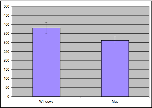
To use the standard error technique, draw a bar chart of the means for each condition, with error bars (whiskers) stretching 1 standard error above and below the top of each bar. If we look at whether those error whiskers **overlap** or are substantially different, then we can make a rough judgement about whether the true means of those conditions are likely to be different. Suppose the error bars overlap - then it's possible that the true means for both conditions are actually the same - in other words, that whether you use the Windows or Mac menubar design makes no difference to the speed of access. But if the error bars do not overlap, then it's likely that the true means are different.
The error bars can also give you a sense of the reliability of your experiment, also called the **statistical power**. If you didn't take enough samples - too few users, or too few trials per user - then your error bars will be large relative to the size of the data. So the error bars may overlap even though there really is a difference between the conditions. The solution is more repetition - more trials and/or more users - in order to increase the reliability of the experiment.
Our hypothesis is that the position of the menubar makes a difference in time. Another way of putting it is that the (noisy) process that produced the Mac access times is **different** from the process that produced the Windows access times. Let's make the hypothesis very specific: that the mean access time for the Mac menu bar is less than the mean access time for the Windows menu bar.
In the presence of randomness, however, we can't really *prove* our hypothesis. Instead, we can only present evidence that it's the best conclusion to draw from all possible other explanations. We have to argue against a skeptic who claims that we're wrong. In this case, the skeptic's position is that the position of the menu bar makes *no* difference; i.e., that the process producing Mac access times and Windows access times is the same process, and in particular that the mean Mac time is equal to the mean Windows time. This hypothesis is called the **null hypothesis**. In a sense, the null hypothesis is the "default" state of the world; our own hypothesis is called the **alternative hypothesis**.
Our goal in hypothesis testing will be to accumulate enough evidence - enough of a difference between Mac times and Windows times - so that we can **reject the null hypothesis** as very unlikely.
Here's the basic process we follow to determine whether the measurements we made support the hypothesis or not.
We summarize the data with a **statistic** (which, by definition, is a function computed from a set of data samples). A common statistic is the mean of the data, but it's not necessarily the only useful one. Depending on what property of the process we're interested in measuring, we may also compute the variance (or standard deviation), or median, or mode (i.e., the most frequent value). Some researchers argue that for human behavior, the median is a better statistic than the mean, because the mean is far more distorted by outliers (people who are very slow or very fast, for example) than the median.
Then we apply a **statistical test** that tells us whether the statistics support our hypothesis. Two common tests for means are the **t test** (which asks whether the mean of one condition is different from the mean of another condition) and **ANOVA** (which asks the same question when we have the means of three or more conditions).
The statistical test produces a **p value**, which is the probability that the difference in statistics that we observed happened purely by chance. Every run of an experiment has random noise; the p value is basically the probability that the means were different only because of these random factors. Thus, if the p value is less than 0.05, then we have a 95% confidence that there really is a difference. (There's a more precise meaning for this, which we'll get to in a bit.)
Here's the basic idea behind statistical testing. We boil all our experimental data down to a single statistic (in this case, we'd want to use the difference between the average Mac time and the average Windows time). If the null hypothesis is true, then this statistic has a certain probability distribution. (In this case, if H0 is true and there's no difference between Windows and Mac menu bars, then our difference in averages should be distributed around 0, with some standard deviation).
So if H0 is really true, we can regard our entire experiment as a single random draw from that distribution. If the statistic we computed turned out to be a typical value for the H0 distribution - really near 0, for example - then we don't have much evidence for arguing that H0 is false. But if the statistic is extreme - far from 0 in this case - then we can **quantify** the likelihood of getting such an extreme result. If only 5% of experiments would produce a result that's at least as extreme, then we say that we reject the null hypothesis - and hence accept the alternative hypothesis H1, which is the one we wanted to prove - at the 5% significance level.
The probability of getting at least as extreme a result given H0 is called the **p value** of the experiment. Small p values are better, because they measure the likelihood of the null hypothesis. Conventionally, the p value must be 5% to be considered **statistically significant**, i.e., enough evidence to reject. But this convention depends on context. An experiment with very few trials (n<10) may be persuasive even if its p value is only 10%. (Note that a paper reviewer would expect you to have a good reason for running so few trials that the standard 5% significance wasn't enough...) Conversely, an experiment with thousands of trials won't be terribly convincing unless its p value is 1% or less.
Keep in mind that **statistical significance does not imply importance**. Suppose the difference between the Mac menu bar and Windows menu bar amounted to only 1 millisecond (out of hundreds of milliseconds of total movement time). A sufficiently large experiment, with enough trials, would be able to detect this difference at the 5% significance level, but the difference is so small that it simply wouldn't be relevant to user interface design.
Hypothesis Testing
Let's return to the example we used in the experiment design reading. Suppose we've conducted an experiment to compare the position of the Mac menubar (flush against the top of the screen) with the Windows menubar (separated from the top by a window title bar). For the moment, let's suppose we used a **between-subjects** design. We recruited users, and each user used only one version of the menu bar, and we'll be comparing different users' times. For simplicity, each user did only one trial, clicking on the menu bar just once while we timed their speed of access. (Doing only one trial is a very unreliable experiment design, and an expensive way to use people, but we'll keep it simple for the moment.) The results of the experiment are shown above (times in milliseconds; note that this is fake, randomly-generated data, and the actual experiment data probably wouldn't look like this). Mac seems to be faster (574 ms on average) than Windows (590 ms). But given the noise in the measurements - some of the Mac trials are actually much slower than some of the Windows trials -- how do we know whether the Mac menubar is really faster? This is the fundamental question underlying statistical analysis: estimating the amount of evidence in support of our hypothesis, even in the presence of noise.Standard Error of the Mean
N = 4: Error bars overlap, so can't conclude anything
N = 10: Error bars are disjoint, so Windows may be different from Mac